
概述
先贴上比赛地址:https://www.kaggle.com/c/nfl-big-data-bowl-2020
比赛大意是在美式橄榄球比赛中🏉,需要对进攻方每一轮跑动推进的码数进行预测,比较在意的是这个问题的评价指标很奇特,用到了分级概率函数,具体见连续分级概率评分,相应的,我们既可以把它处理成199个分类的多分类问题,也可以处理成回归问题,这里操作的空间就很大了。同时最后的B榜来源于12月到1月即将举办的比赛,是未来的数据,这带来了更大的挑战。
此外该赛题是kernal based,选手最后提交的是一个.ipynb的可运行jupyter文件,也就是说每次预测会重新跑这段代码,训练新的模型并进行预测,而比赛对应的训练集也会随着比赛的进行,B榜的更新而更新,会把新的比赛数据加入到训练集之中,这带来的挑战是需要我们为增量的数据预留好空间和时间复杂度(单个kernal可执行时间需小于4小时,最大内存16G)
DATA
先附上原始数据的数据词典,对于美式橄榄球不熟悉的可以参考 美式橄榄球
数据源:https://www.kaggle.com/c/nfl-big-data-bowl-2020/data
GameId- a unique game identifier 比赛IDPlayId- a unique play identifier 一场比赛中所有play的ID(每次play都有可能得分)Team- home or away 队名X- player position along the long axis of the field. See figure below.Y- player position along the short axis of the field. See figure below.
NFL和NCAA使用的标准球场是一个长360英尺(120码或109.7米)、宽160英尺(53.33码或48.8米)的长方形草坪(有些室内赛会使用仿草地毯),较长的边界称为边线(sideline),较短的边界称为端线(end line)。端线前的标示线称为得分线(goal line),球场每侧端线与得分线之间有一个纵深10码(9.1米)的得分区叫做端区(end zone,也称达阵区),端区的四角各有一个约有1英尺长的橙色长方体标柱(pylon)。两侧得分线相距100码(91.44米),之间的区域也就是比赛区(playing field)。比赛区上距离得分线每5码(4.6米)距离标划一条码线(yard line,或称5码线),每10码标示数字,直到50码线到达中场(midfield)。在球场中间和两侧与边线平行排列划有横向的短标示线,称为码标(hash marks,或称整码线),其中接近边线的码标线称为界内线(inbounds line)。任何球员都必须在码标线上或之间进行发球。
S- speed in yards/second 此时的速度A- acceleration in yards/second^2 加速度Dis- distance traveled from prior time point, in yardsOrientation- orientation of player (deg) 玩家面对的方向Dir- angle of player motion (deg) 玩家移动的方向
NflId- a unique identifier of the player 运动员IDDisplayName- player’s name 运动员nameJerseyNumber- jersey number 运动员号码Season- year of the seasonYardLine- the yard line of the line of scrimmage 发球的码线Quarter- game quarter (1-5, 5 == overtime) 比赛所处的时间GameClock- time on the game clockPossessionTeam- team with possession 当前拥有控球权的队伍Down- the down (1-4)进攻方有四次机会向前方(防守方的端区)累计推进10码,每次机会称为一“档” 进攻(down,即被对方拦截放倒一次的机会)。当进攻方成功的在四档进攻内推进了10码以上,便可获得新的四档进攻机会——称为获得新的 “首档”(1st down,也称首攻)。通过不断获得新的首攻,进攻方可以进行连续的系列进攻向前不断推进,直至得分。而防守方的目的也很简单——就是尽可能阻止对方在四档进攻内推进足够的距离,逼迫其交换控球权。
Distance- yards needed for a first down 距离新的首攻所需要的码数FieldPosition- which side of the field the play is happening on play发生在哪个球队的半场HomeScoreBeforePlay- home team score before play started 主队已经获得的比分VisitorScoreBeforePlay- visitor team score before play started 客队已经获得的比分NflIdRusher- theNflIdof the rushing player 进攻方持球选手IDOffenseFormation- offense formationOffensePersonnel- offensive team positional grouping 进攻队员DefendersInTheBox- number of defenders lined up near the line of scrimmage, spanning the width of the offensive lineDefensePersonnel- defensive team positional grouping 防守队员PlayDirection- direction the play is headedTimeHandoff- UTC time of the handoff 传球时间TimeSnap- UTC time of the snap 发球的时间Yards- the yardage gained on the play (you are predicting this) 得分,即最后预测的yPlayerHeight- player height (ft-in)PlayerWeight- player weight (lbs)PlayerBirthDate- birth date (mm/dd/yyyy)PlayerCollegeName- where the player attended collegePosition- the player’s position (the specific role on the field that they typically play)HomeTeamAbbr- home team abbreviation 主队缩写VisitorTeamAbbr- visitor team abbreviationWeek- week into the season 赛季的第几周Stadium- stadium where the game is being playedLocation- city where the game is being playerStadiumType- description of the stadium environment 体育馆类型Turf- description of the field surface 场地类型GameWeather- description of the game weatherTemperature- temperature (deg F)Humidity- humidity 湿度WindSpeed- wind speed in miles/hourWindDirection- wind direction
难点
play的特征和每个球员的特征如何统一进模型中
NN可以对不同size 的特征进行处理,可以分别将球员特征进行embeding
play的特征中加入rusher的特征作为球员特征
play的特征中加入每一个球员的所有特征,不建议(球员特征多的时候*22 引入大量噪声),更好的方案是对球员进行聚合(agg)形成特征
多分类问题如何形成评价指标
连续分级概率评分(Continuous Ranked Probability Score, CRPS),按CRPS评价概率模型所得的(优劣)结果与按MAE评价概率模型的数学期望所得的结果等价,train model时用mae
值得注意的是sklearn中的MAE是负值,原因:因为有些score是越大越好,比如roc_auc,但有些越小越好比如各种loss,为了统一,sklearn为最小化的值加了负号转化为最大化的问题,这里需要相应地修改网格里的初始化参数
整个数据集虽然有五十几万,但每场play都对应了22个球员,整理下来play的数据量只有23171 * 72,会造成过拟合,怎么避免
预测上的难点,最后的B榜训练集会加入未来一个月新的比赛数据,kernal based比赛需要做好时间和空间复杂度的控制
关于运动员的运动方向,进攻方可能向左可能向右,此时需要对yard进行转换,处理时有个trick是将X,y,角度都进行翻转,保证进攻方的方向始终是一致的以便于特征的处理
EDA
梳理一下问题其实就是,一个rusher,10个队友,11个防守方的竞赛,rusher会尽一切努力冲破防守方防线,对应地防守方会不顾一切跑向rusher以阻止他,队友也需要跑向rusher以协助进攻,因此不难发现距离的特征会很重要。故我们的特征工程主要围绕这一变量展开:
- 将进攻方向进行统一,转换对应的yardline、x、y、orientation、direction
- 每个play加入rusher的相关特征
- 增加球员特征的统计特征agg
min', 'max', 'mean', 'std', 'skew', 'median', q80, q30, pd.DataFrame.kurt, 'mad',np.ptp - 将球员分为进攻方和防守方,分别进行距离rusher距离、x、y的聚合统计
- 尝试穿越特征:计算队伍历史场均推进,后在lb上未有明显提高,放弃(考虑效果不好的原因:1.测试集队伍和训练集可能不同,有缺失值;2.场均推进受进攻方和防守方共同影响,仅仅根据进攻方计算的推进距离会有失真)
第一名的特征思路总结地更好,见https://www.kaggle.com/c/nfl-big-data-bowl-2020/discussion/119400#latest-685747
model
NN:
分别处理category和dense的NN,效果一般
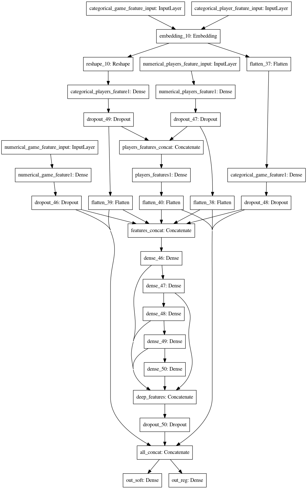
用最简单的全连接的NN,自定义损失函数,通过early stopping和dropout降低过拟合
class CRPSCallback(Callback):

    def __init__(self, validation, predict_batch_size=20, include_on_batch=False):
        super(CRPSCallback, self).__init__()
        self.validation = validation
        self.predict_batch_size = predict_batch_size
        self.include_on_batch = include_on_batch

    def on_batch_begin(self, batch, logs={}):
        pass

    def on_train_begin(self, logs={}):
        if not ('CRPS_score_val' in self.params['metrics']):
            self.params['metrics'].append('CRPS_score_val')

    def on_batch_end(self, batch, logs={}):
        if (self.include_on_batch):
            logs['CRPS_score_val'] = float('-inf')

    def on_epoch_end(self, epoch, logs={}):
        logs['CRPS_score_val'] = float('-inf')

        if (self.validation):
            X_valid, y_valid = self.validation[0], self.validation[1]
            y_pred = self.model.predict(X_valid)
            y_true = np.clip(np.cumsum(y_valid, axis=1), 0, 1)
            y_pred = np.clip(np.cumsum(y_pred, axis=1), 0, 1)
            val_s = ((y_true - y_pred) ** 2).sum(axis=1).sum(axis=0) / (199 * X_valid.shape[0])
            val_s = np.round(val_s, 8)
            logs['CRPS_score_val'] = val_s

def get_model(x_tr, y_tr, x_val, y_val):
    inp = Input(shape=(x_tr.shape[1],))
    # x = Dense(2048, input_dim=X.shape[1], activation='elu')(inp)
    # x = BatchNormalization()(x)
    # x = Dropout(0.5)(x)
    # x = Dense(1024, activation='elu')(x)
    x = Dense(1024, input_dim=X.shape[1], activation='elu')(inp)
    x = BatchNormalization()(x)
    x = Dropout(0.5)(x)
    x = Dense(512, activation='elu')(x)
    x = BatchNormalization()(x)
    x = Dropout(0.5)(x)
    x = Dense(256, activation='elu')(x)
    x = BatchNormalization()(x)
    x = Dropout(0.5)(x)
    if classify_type < 128:
        x = Dense(256, activation='elu')(x)
        x = BatchNormalization()(x)
        x = Dropout(0.5)(x)

    out = Dense(classify_type, activation='softmax')(x)
    model = Model(inp, out)
    optadam = Adam(lr=0.001)
    model.compile(optimizer=optadam, loss='categorical_crossentropy', metrics=[])

    es = EarlyStopping(monitor='CRPS_score_val',
                       mode='min',
                       restore_best_weights=True,
                       verbose=False,
                       patience=80)

    mc = ModelCheckpoint('best_model.h5', monitor='CRPS_score_val', mode='min',
                         save_best_only=True, verbose=False, save_weights_only=True)

    bsz = 1024
    steps = x_tr.shape[0] / bsz

    model.fit(x_tr, y_tr, callbacks=[CRPSCallback(validation=(x_val, y_val)), es, mc], epochs=100, batch_size=bsz,
              verbose=False)
    model.load_weights("best_model.h5")

    y_pred = model.predict(x_val)
    y_valid = y_val
    y_true = np.clip(np.cumsum(y_valid, axis=1), 0, 1)
    y_pred = np.clip(np.cumsum(y_pred, axis=1), 0, 1)
    val_s = ((y_true - y_pred) ** 2).sum(axis=1).sum(axis=0) / (199 * x_val.shape[0])
    crps = np.round(val_s, 8)
    gc.collect()

    return model, crps
Lgbm:
预测多标签方法:最本质的区别在于这里的多标签概率的平滑怎么做,第一种直接用lgbm的api意味着让程序自动进行平滑,而第二种手动展开则只通过得到的预测值,自己制定规则展开,第三种介于一二两种之间,通过手动制定分桶的规则,在每个分桶中自动进行平滑。最后采取了第一种方式。直接用lgbm的api:https://www.kaggle.com/enzoamp/nfl-lightgbm/code
'objective':'multiclass',
"metric": 'multi_logloss',
'num_class': 199,
用LGBMRegressor,得到预测值后加函数展开, https://www.kaggle.com/newbielch/lgbm-regression-view
https://www.kaggle.com/apiao1/model-lgbm-regression/notebook?scriptVersionId=23357454
V4 cv:0.01360 lb:0.01412(不及原文的成绩,原文的cv0.01349,lb0.01401) 应该过拟合很严重,调参应该有较好结果LGBMClassifier + 平滑, https://www.kaggle.com/mrkmakr/lgbm-multiple-classifier
https://www.kaggle.com/apiao1/model-lgbm-multipleclassifier?scriptVersionId=23397574
V7 效果不好,cv:0.020105, lb:0.02159 ,猜测哪里有bug,(原文:cv:0.013140205432501861,lb:0.01384)
RF:
model = RandomForestRegressor(bootstrap=False, max_features=0.3, min_samples_leaf=15, min_samples_split=7,n_estimators=250, n_jobs=-1, random_state=2019)
model.fit(tr_x, tr_y)
关于ensemble:
- 效果不理想,采用NN和lgbm的stacking分数与单模型NN相同
- 最后的提交用了两个版本,NN-传统的blending,NN和lgb-简单的stacking
trick
推进距离(Yards)一定小于此时距离得分的距离(Yards_limit),据此进行后验的处理
对训练集统计发现样本标签的分布为-14至99,在-99至-14区间没有任何正例样本,固把预测类别标签缩小至-14到99的范围内
NN对数据的变化很敏感,所以可以尝试多次k折的数据分割,用不同的随机数种子去做,本地得到的cv更低
losses = []
  models = []
  mean_crps_csv = []

  for k in range(5):
      kfold = KFold(9, random_state=2019 + 17 * k, shuffle=True)
      j = 0
      crps_csv = []
      for k_fold, (tr_inds, val_inds) in enumerate(kfold.split(yards)):
          j += 1
          if j > 3:
              break
          tr_x, tr_y = X[tr_inds], y[tr_inds]
          val_x, val_y = X[val_inds], y[val_inds]
          model, crps = get_model(tr_x, tr_y, val_x, val_y)
          models.append(model)
          # print("the %d fold crps is %f" % ((k_fold + 1), crps))
          crps_csv.append(crps)
      mean_crps_csv.append(np.mean(crps_csv))
      print("9 folder crps is %f" % np.mean(crps_csv))

  print("mean crps is %f" % np.mean(mean_crps_csv))
用贝叶斯调参效果比传统的网格和优化后的启发式网格效果都要更好
What didn’t work
- 没有尝试用CNN处理(事实上确实有效)
- 只计算了球员们的相对距离,没有将位置关系和速度加速度转化成相对值,只是做了方向度量上的统一
- 没有找到一个稳定的cv评价方式,cv与lb之间变化不一致,导致后期筛选特征很没谱非常乏力
- 不同年份的数据权重,2018年数据权重高于2017年数据。
- 不同的数据划分方式,尝试根据比赛年份进行groupKfold
Thinking
- 打kaggle确实要组队,一个人又要调模型又要做特征真的太花精力了,而且缺少人一起讨论,后期思维就局限了,不利于提升
- 队友也挺重要的,这次比赛的队友白天都在上班太忙了Orz
- 一个好的baseline能省去不少功夫,由于参加的早(距结束一个月开始做),中间换了好多baseline浪费了很多时间,推荐距离结束14-21天开始为宜
- 特征为王
- 事先找到一个和lb变化一致的cv事半功倍
- kaggle 的代码工程化思维实在太弱了,大部分都是面向过程,改baseline的时候实在太难过了
算是kaggle的首战吧,确实投入了很多时间,之前一直处于银牌,很可惜lb最后一天掉出了银牌区,就差两名,最后一天也奋战到深夜(第二天还要早起确定最后的提交),把我能尝试的都尝试了,算是尽了人事,静待最后的结果吧~
1月6日B榜最后的结果,届时大家会开源自己的代码,到时候进一步对照代码学习提升,明天开始和新队友打新的比赛啦
冠军方案小结
刚看了几个高分的方案,其中冠军方案用了CNN进行实现,而且不是传统意义上对图像进行处理,令人印象深刻。https://www.kaggle.com/c/nfl-big-data-bowl-2020/discussion/119400
再梳理一遍整个大赛的动机:
- 一个冲刺者,其目标是尽可能向前冲
- 11名试图阻止冲锋队的防守球员
- 剩下的10名进攻球员试图阻止防守者阻止或应对冲锋队员
从中可以得到对预测结果影响较大的排序依次为:rusher -> defender -> offender。画出某个play时场上队员的分布如下: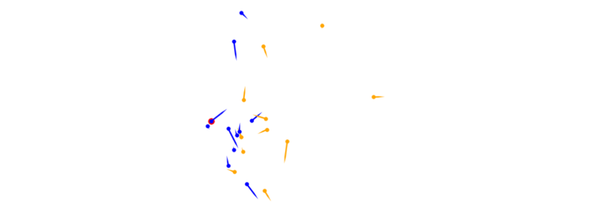
在比赛的前期只考虑了rusher与defender 的特征,那么它看起来就像是一个简单的游戏,如下图,其中一个玩家试图逃跑,而其他11个玩家试图抓住他。我们假设在比赛开始时,无论防守者的位置如何,每位防守者都将集中精力尽快阻止进攻者,而每位防守者都有机会做到这一点。防守者铲球的机会(以及铲球的估计位置)取决于他们的相对位置,移动速度和运动方向。通过使用相对位置和速度在各个防御者上进行卷积的想法,然后在顶部应用池化压缩。

之后加入了队友相关的特征,也采用类似的处理。
模型结构
最终的模型结构CNN如下:
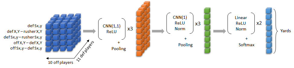
将所有的数据重塑为进攻与防守的张量,且仅用了5个相关的特征,分别是:防守方的加速度、防守方相对于rusher的加速度、位置,进攻方相对于防守方的位置、加速度。考虑到如此处理后整个初始数据集是个10*11*5的三维矩阵,通过CNN的特性恰到好处的进行了压缩与Embeding。
So the first block of convolutions learns to work with defense-offense pairs of players, using geometric features relative to rusher. The combination of multiple layers and activations before pooling was important to capture the trends properly. The second block of convolutions learns the necessary information per defense player before the aggregation. And the third block simply consists of dense layers and the usual things around them. 3 out of 5 input vectors do not depend on the offense player, hence they are constant across “off” dimension of the tensor.
在pooling部分用的是加权组合,即0.7*maxpooling + 0.3 * avgpooling
数据增强和TTA
对我们来说真正有效的方法是为Y坐标添加增强和TTA。我们假设在镜像的世界中,运行将具有相同的结果。对于训练,我们应用50%增强来翻转Y坐标(以及由此产生的所有各个相对特征)。对于TTA,我们做同样的事情,我们有50-50的翻转和非翻转推论混合。
代码优化
我们很早就决定最好在内核中进行所有拟合,特别是因为在重新运行中我们还有2019年可用的数据。因此,我们还决定早点花时间优化运行时间,因为我们也知道,在拟合神经网络时,用不同的种子打包多次运行非常重要,因为这通常会显着提高准确性,并消除了一些运气因素。
如上所述,我们使用Pytorch进行拟合。Kaggle内核有2个具有4个内核的CPU,其中两个内核是真实内核,另外两个是用于超线程的虚拟内核。一次运行使用所有4个内核时,就运行时而言,它并不是最佳选择,因为您无法在合适的情况下对每个操作进行多处理。因此,我们要做的是禁用Python的所有多线程和多处理(MKL,Pytorch等),并在bag级别上进行手动多处理。这意味着我们可以同时拟合4个模型,与在所有4个内核上拟合单个模型相比,可以获得更多的运行时间。
我们的最终潜艇每个保守地适合8个模型,潜艇的总运行时间低于8500秒。
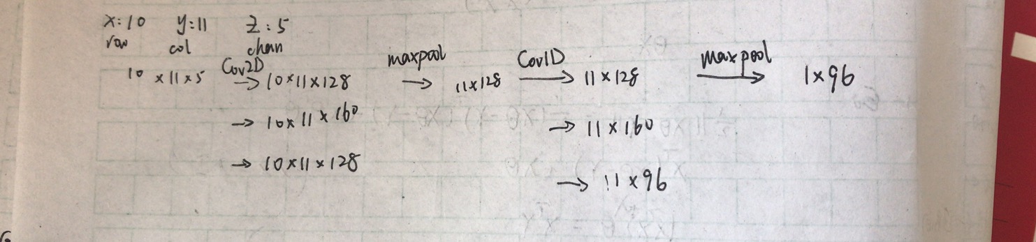
CNN伪代码
评论部分的伪代码,源代码尚未开源,已开源,见更新部分:
inputdenseplayers = Input(shape=(11,10,10), name = "numericalplayersfeature_input") |
- we have another BN after the first pooling and before the first Conv1D
- The Conv1D dimensions are 160-96-96 (I wrote that wrongly below)
- After the very last linear layer we have Relu-LayerNorm-Dropout(0.3)
- There is no regression output (and loss is crps afterwards)
对应上面的伪代码和整个模型的架构,其维度变化如下所示:
1.16更新
冠军方案的源代码已开源:https://www.kaggle.com/philippsinger/nfl-playing-surface-analytics-the-zoo
真的是让人膜拜的方案,遗憾的是他们的方案在b榜运行失败了,没有最终成绩。更让我意识到kernal based比赛代码鲁棒性的重要性。
最后的b榜结果也出来了,6%铜牌,可惜了差一点银牌,再接再厉💪